In this post I want to talk about linear regression cost function and the relationship between solving using normal equations and gradient descent when there is more features than samples in our dataset.

I belonged to a group of people thas was studiying the book “Introduction to statistical learning with R” and in the chapter 3 it talk about linear regression and the authors give the following example:

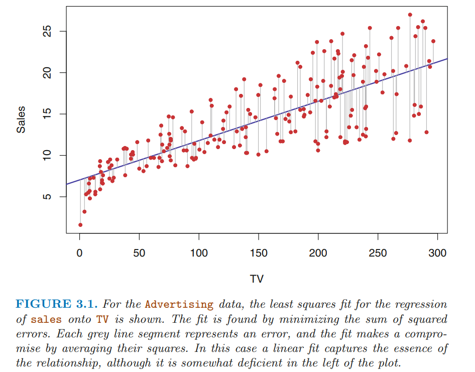
Then they give us the loss function

$RSS$ is a funtion of the dataset, different datasets give us different cost functions. In this case is a function of two parameters $\beta_{1}$ y $\beta_{2}$.

Then they plot the three dimensional cost function in this way

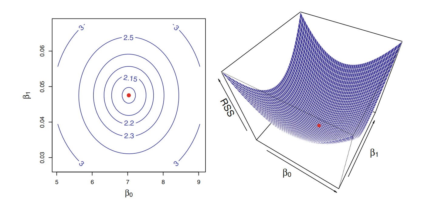
We can see that the function has only one minimum. Equating the gradient of the cost function to zero and doing some calculation we can arrive at this expression:

But we know that if there is more parameters than equations then there are infinite solutions.

The question is given that analytically there are infinite solutions, what happen if I try to solve using gradient descent when I have a dataset with 999 samples and 1000 features each? The logic said this method has to suffer the same problems as normal equations, but given that we allways have in our minds this perfect paraboloid we think that gradient descent has to find a single solution because the paraboliod has only one minimun. But this is not true when there is more parametters than equations, but given that it’s is impossible to plot that function when there are more than two parameters I will plot the function in three dimentions with different amount of samples. At the end I will share the code to plot the cost function depending of the amount of samples.

One sample two features

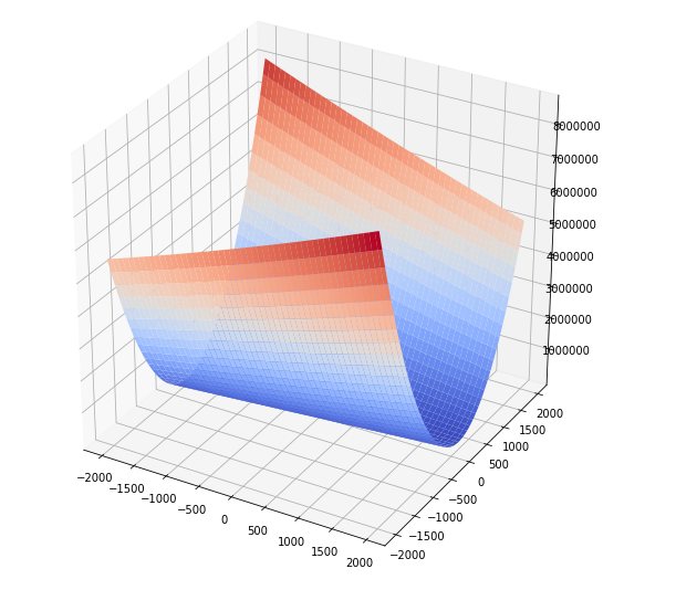
This is what happen whe we have more features than samples, there is a infinite subspace where the cost function reach the minimun and this is coherent with what happend with normal equations. I can reach infinite solutions depending from what point the gradient descent start.

Two samples two features

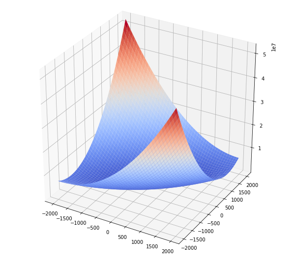
In this case the function has one minimun as normal equations, but this is not a perfect paraboloid.

Ten samples two features

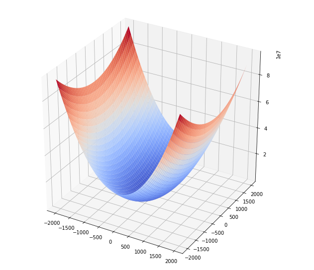
We can see how the cost function start to present rotational symmetry.

One hundred samples two features

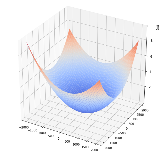
It surprise me, why the cost function start to present aparently rotational symmetry when we have a lot of samples? I don’t have an answer yet.

This analysis gave to me an insight that the cost function in linear regression is not a symmetric perfect function it depends of the size of our dataset. And when we have more features than equations the cost funcion has an infinite subspace where the function reach the same minimun causing gradient descent to suffer the same problem as normal equations. This is beautiful for me because given two very different methods to solve linear regression both method behave in the same way “Math is coherent”.

Code

In this Notebook you can find the code to generate the plots.